有限差分方法近似函数导数

Tintingo / 2022-02-26

Categories: WaveEquation / Tags: WaveEquation, FDM / Word Count: 1242

有限差分法是求解偏微分方程的主要数值方法之一，其基本思想是用离散的只含有有限个未知量的差分方程组去近似代替连续变量的微分方程和定解条件，并把差分方程组的解作为微分方程定解问题的近似解。用差分法将连续问题离散化的主要步骤如下：

对求解区域作网格剖分，用有限的网格节点代替连续区域。
构造差分格式，即通过适当的方法将微分方程离散化，导出线性方程组。
对离散点上的近似值进行插值逼近，得到整个区域上的近似解。

有限差分法把控制方程中的导数用网格节点上的函数值的差商代替以进行离散，从而建立以网格节点上的值为未知数的代数方程组。

一阶导数的有限差分近似

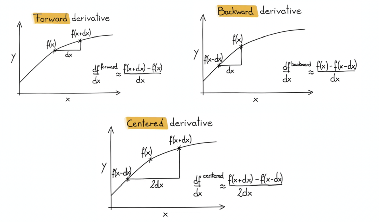
三种一阶导数的差商形式

需要说明的是，利用有限差分离散偏微分方程的方法是多种多样的，即使对同一个方程也可以构造不同的差分格式。首先，使用网格节点上函数值的差商代替导数时，就可以分为前向差商、中心差商、后向差商等方法。

${\frac{d f}{d x}}^{f o r w a r d} \approx \frac{f (x + d x) - (x)}{d x}$

${\frac{d f}{d x}}^{c e n t e r} \approx \frac{f (x + d x) - (x - d x)}{2 d x}$

${\frac{d f}{d x}}^{b a c k w a r d} \approx \frac{f (x) - (x - d x)}{d x}$

可以从下图中清楚地看到三种情况的几何意义。

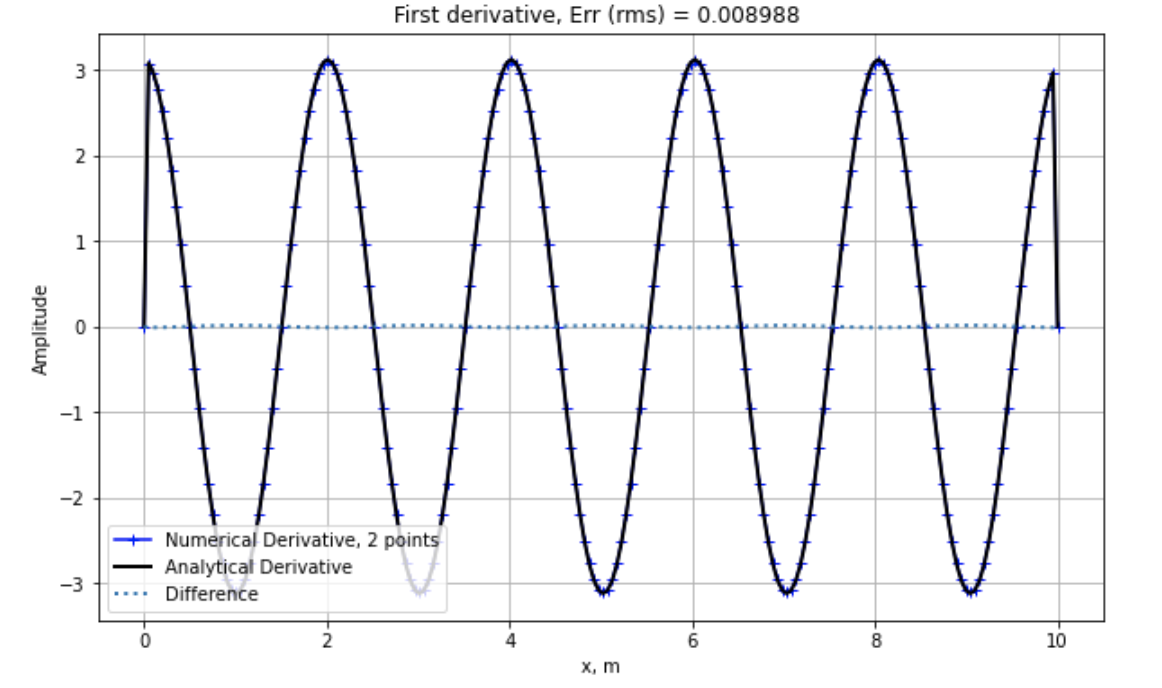
当 $d x$ 足够小时，我们就可以认为使用函数点与周围点的差商能够近似代替该点的导数。下面使用 python 代码说明中心差商对导数的近似。

python 计算数值一阶导数 – 中心差商

对于函数： $\begin{matrix} (1) & f (x) = s i n (k x) \end{matrix}$ 其中 $k$ 为波数： $k = 2 π / λ$ ，可以很容易求得该函数的一阶导数作为中心差商的验证： $\begin{matrix} (2) & f^{'} (x) = k c o s (k x) \end{matrix}$ 函数在 $x$ 点处的中心差商表示为：

$\begin{matrix} (3) & f^{'} (x) \approx \frac{f (x + d x) - f (x - d x)}{2 d x} \end{matrix}$

# Import Libraries
import numpy as np
from math import *
import matplotlib.pyplot as plt

# Initial parameters
xmax = 10.0                     # physical domain (m)
nx = 200                        # number of samples    
dx = xmax/(nx-1)                # grid increment dx (m)
x  = np.linspace(0,xmax,nx)     # space coordinates

# Initialization of sin function
l = 40*dx     # wavelength
k = 2*pi/l    # wavenumber
f = np.sin(k*x)

# First derivative with two points

# Initiation of numerical and analytical derivatives 
nder=np.zeros(nx)          # numerical derivative
ader=np.zeros(nx)          # analytical derivative

# Numerical derivative of the given function
for i in range (1, nx-1):
    nder[i]=(f[i+1]-f[i-1])/(2*dx)

# Analytical derivative of the given function
ader= k * np.cos(k*x)   
# Exclude boundaries
ader[0]=0.
ader[nx-1]=0.

# Error (rms) 
rms = np.sqrt(np.mean((nder-ader)**2))

# Plotting 
# ----------------------------------------------------------------
plt.figure(figsize=(10,6))
plt.plot (x, nder,label="Numerical Derivative, 2 points", marker='+', color="blue")
plt.plot (x, ader, label="Analytical Derivative", lw=2, ls="-",color="black")
plt.plot (x, nder-ader, label="Difference", lw=2, ls=":")
plt.title("First derivative, Err (rms) = %.6f " % (rms) )
plt.xlabel('x, m')
plt.ylabel('Amplitude')
plt.legend(loc='lower left')
plt.grid()
plt.show()

二阶导数的有限差分近似

使用与上一节中一阶导数相同的推导思路，若使用 $x - d x$ , $x$ , $x + d x$ 三点计算差商，则二阶导数的三点有限差分近似可以写为：

$\begin{matrix} (4) & f_{n u m}^{''} (x) = \frac{f (x + d x) - 2 f (x) + f (x - d x)}{d x^{2}} \end{matrix}$

以及如果使用 $x - 2 d x$ , $x - d x$ , $x$ , $x + d x$ , $x + 2 d x$ 五点计算差商，则二阶导数的五点有限差分近似可以写为： $\begin{matrix} (5) & f^{''} (x) = \frac{- \frac{1}{12} f (x - 2 d x) + \frac{4}{3} f (x - d x) - \frac{5}{2} f (x) + \frac{4}{3} f (x + d x) - \frac{1}{12} f (x + 2 d x)}{d x^{2}} \end{matrix}$

python 计算数值二阶导数 – 三点及五点差商

对于 Gaussian 函数：

$\begin{matrix} (6) & f (x) = \frac{1}{\sqrt{2 π a}} e^{- \frac{(x - x_{0})^{2}}{2 a}} \end{matrix}$

对该函数进行二阶求导，可以得到：

\begin{matrix} (7) & f^{''} (x) = \frac{1}{\sqrt{2 π a}} (\frac{(x - x_{0})^{2}}{a^{2}} - \frac{1}{a}) e^{- \frac{(x - x_{0})^{2}}{2 a}} \end{matrix}

# Initialization 
xmax=10.0       # physical domain (m)
nx=100          # number of space samples
a=.25           # exponent of Gaussian function    
dx=xmax/(nx-1)  # Grid spacing dx (m)
x0 = xmax/2     # Center of Gaussian function x0 (m)

x=np.linspace(0,xmax,nx)   # defining space variable

# Initialization of Gaussian function           
f=(1./sqrt(2*pi*a))*np.exp(-(((x-x0)**2)/(2*a)))

# Second derivative with three-point operator

# Initiation of numerical and analytical derivatives 
nder3=np.zeros(nx)          # numerical derivative
ader=np.zeros(nx)          # analytical derivative

# Numerical second derivative of the given function 
for i in range (1, nx-1):
    nder3[i]=(f[i+1] - 2*f[i] + f[i-1])/(dx**2)

# Analytical second derivative of the Gaissian function
ader=1./sqrt(2*pi*a)*((x-x0)**2/a**2 -1/a)*np.exp(-1/(2*a)*(x-x0)**2)
# Exclude boundaries
ader[0]=0.
ader[nx-1]=0.

# Calculate rms error of numerical derivative
rms = np.sqrt(np.mean((nder3-ader)**2))

# Plotting 
plt.figure(figsize=(10,6))
plt.plot (x, nder3,label="Numerical Derivative, 3 points", lw=2, color="violet")
plt.plot (x, ader, label="Analytical Derivative", lw=2, ls="--")
plt.plot (x, nder3-ader, label="Difference", lw=2, ls=":")
plt.title("Second derivative, Err (rms) = %.6f " % (rms) )
plt.xlabel('x, m')
plt.ylabel('Amplitude')
plt.legend(loc='lower left')
plt.grid()
plt.show()

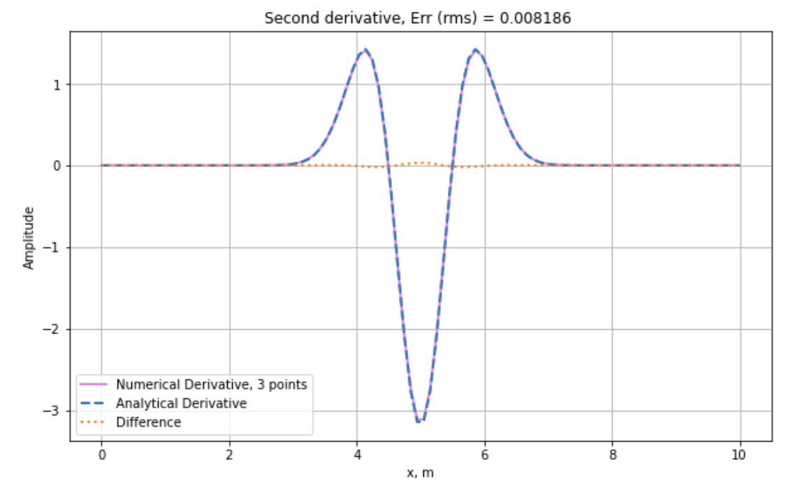
到这里我们就使用三点差商形式求得了 Gaussian 函数的数值二阶导数，与解析得到的二阶导数相比，误差 rms 为 0.008186. 保持其他参数不变，我们使用五点差商形式看看精度如何。

# Second derivative with five points Q: five points = fourth-order?

# Initialisation of derivative
nder5=np.zeros(nx) 

# Calculation of 2nd derivative  
for i in range (2, nx-2):
    nder5[i] = (-1./12 * f[i - 2] + 4./3  * f[i - 1] - 5./2 * f[i] \
                       +4./3  * f[i + 1] - 1./12  * f[i + 2]) / dx ** 2
    
# Exclude boundaries
ader[1]=0.
ader[nx-2]=0.
    
# Calculate rms error of numerical derivative
rms=rms*0
rms = np.sqrt(np.mean((nder5-ader)**2))

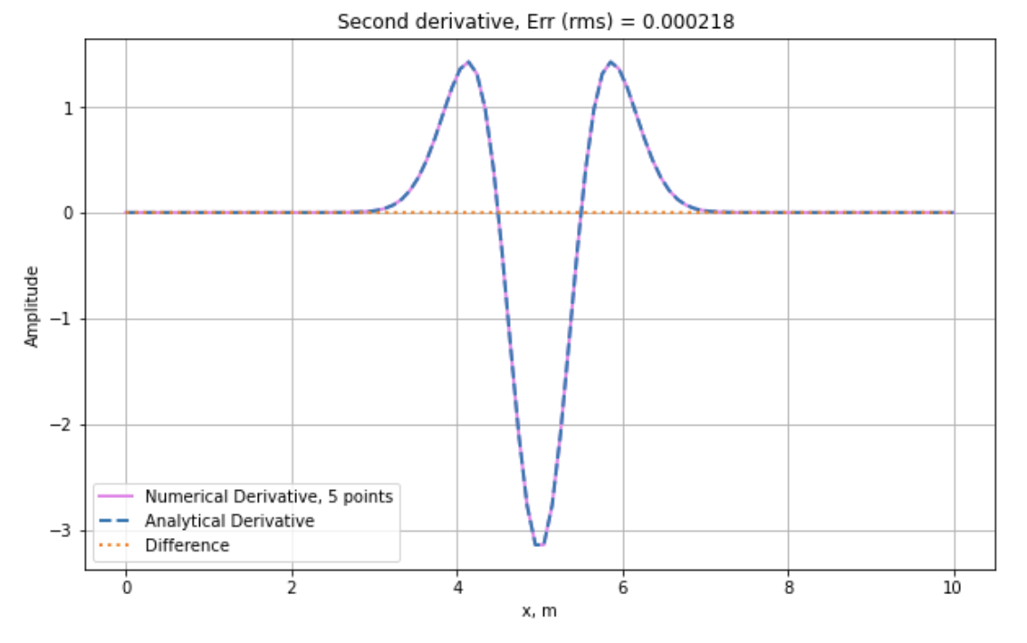
可以发现五点差商形式的误差 rms 为 0.000218，比三点差商形式高出一个数量级。